Over the past year I’ve had the opportunity to use Telegraf, InfluxDB, and Grafana as part of my day job. During this time I’ve stumbled into many problems which I’ve had to work out solutions to, so I thought I would share them since real world examples using InfluxDB, expecially version 2 and Flux, are few and far between.
In these examples I’m using InfluxDB version 2.0.4. There are differences (bugs?) between how version 1 and 2 deal with aggregation and grouping which results in me having to use experimental time functions with version 2 in order to get the same results I was used to getting with version 1.
Downsampling Data
Below is a InfluxDB task (written in Flux) which downsamples data from the Telegraf CPU plugin into 5 minute sampled. Telegraf is configured to sample data each minute (the default interval is 10s but this is just far too fine-grained for my needs).
1
2
3
4
5
6
7
8
9
10
11
12
13
14
15
16
17
18
import "math"
import "date"
import "experimental"

interval = 5m
startRange = 1h
start = date.truncate(t: experimental.subDuration(d: startRange, from: now()), unit: interval)
stop = date.truncate(t: experimental.addDuration(d: interval, to: now()), unit: interval)

from(bucket: "telegraf/autogen")
	|> range(start: start, stop: stop)
	|> filter(fn: (r) => (r._measurement == "cpu"))
	|> aggregateWindow(every: interval, fn: mean)
	|> filter(fn: (r) => (exists r._value))
	|> map(fn: (r) => ({r with _value: math.round(x: r._value * 100.0) / 100.0}))
	|> timeShift(duration: duration(v: "-" + string(v: interval)))
	|> set(key: "_measurement", value: "cpu_" + string(v: interval))
	|> to(bucket: "telegraf/downsampled")
The same code can be used to create windows of any size just by changin the interval variable. The startRange variable is used to set how far back to aggregate data, the longer the time window, the longer the task will take to run.
For example, below are the values required to create data in 1 hour windows processing the past 3 hours.
1
2
interval = 1h
startRange = 3h
For my requirements I downsample to 5 minute, 1 hour, and 1 day measurements.
Some other quick points to note:
- The start and stop variables are used to create neatly aligned time windows as otherwise the results at either end can get funky.
-
The second filter function is required to ensure we don’t try to perform futher operations on null values, as this causes an error.
-
The map function is used to round number down to 2 decimal places. Using the round funtion by itself would result in only whole numbers, which is why we multiply and then divide.
-
The timeshift funtion is used to get the same results in InfluxDB v2 as we would with the same query in InfluxDB v1.
- The set and to functions are used to specifiy the new name for the downsampled measurement and speccifiy which bucket to put the data in.
Grafana Query
One of the first issues I hit when I started using Grafana with influxDB was related to performance when the selected time range in Grafana was too large while the granularity of the InfluxDB data was too fine. To impvoe the performance I created a dynmanic internal variable (this sets the size of the influxDB aggregation window) and I dynamically selected the downsampled measurement, both were based on the time range selected in Grafana.
By using this technique I can nagivate from a 1 hour time range all the way out to a 2 year time range with no performance issues.
1
2
3
4
5
6
7
8
9
10
11
12
13
14
15
16
17
18
19
20
21
22
23
24
25
26
27
28
29
30
31
32
33
34
35
import "experimental"
import "date"
import "strings"

// Name of the bucket to read from
bucket = "telegraf/downsampled"

// Duration of the selected time window in days
duration = (uint(v: v.timeRangeStop) - uint(v: v.timeRangeStart)) / uint(v: 86400000000000)

// Based on the duration, select an approprate interval size
interval = if duration <= 1 then 5m else
           if duration <= 3 then 10m else
           if duration <= 7 then 30m else
           if duration <= 30 then 2h else
           if duration <= 60 then 3h else
           if duration <= 90 then 6h
           else 1d

// Based on the duration, select which downsampled measurement to use
measurement = if duration <= 60 then "cpu_5m"
    else if duration <= 365 then "cpu_1h"
    else "cpu_1d"

// InfluxDB v2 fixes (these were not required with InfluxDB v1)
fixedStart = date.truncate(t: experimental.subDuration(d: interval, from: v.timeRangeStart), unit: interval)
fixedStop = date.truncate(t: experimental.addDuration(d: interval, to: v.timeRangeStop), unit: interval)

from(bucket: bucket)
  |> range(start: fixedStart, stop:v.timeRangeStop)
  |> filter(fn: (r) => r._measurement == measurement and (r._field == "usage_system" or r._field == "usage_user" or r._field == "usage_iowait" or r._field == "usage_steal" or r._field == "usage_guest" or r._field == "usage_irq"))
  |> filter(fn: (r) => r.cpu == "cpu-total")
  |> filter(fn: (r) => (r["host"] =~ /^$host$/ and r["dc"] =~ /${datacenter:regex}/))
  |> keep(columns: ["_time","_start", "_stop", "_field", "_value"])
  |> aggregateWindow(every: interval, fn: mean)
-
Having the measurement name dynamic means it’s best to drop the measurement name from the final output or else it will mess with any Grafana transformations and overrides. In the example I have given I have not dropped the measurement, instead I’ve specified which columns to keep, with the same end result.
-
The host and dc values are derived from Grafana dashboard variables.
-
Using functions from the experimental package is probably not the best idea as they are liable to change / break / be removed in future InfluxDB versions.
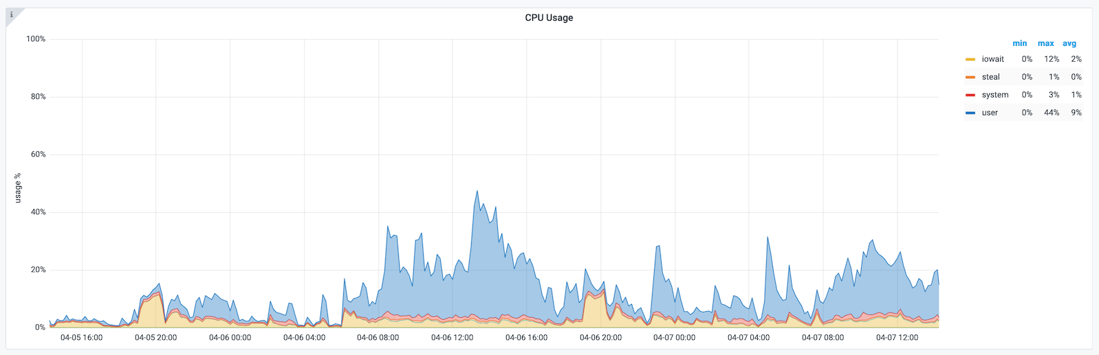
Below is a screenshot from Grafana showing the output of the above query.